Create an iOS application using machine learning

Introduction
Prerequisites
But first of all, what is machine learning?
Secondly, what algorithm will be used?
Project setup
Building the CNN
Transfer learning
Convert to MLModel
iOS application with MLModel
Conclusion
References:

Introduction

We are lucky enough to be living in an era of exponential technology growth. We are lucky enough to witness the transition from yesterday’s technology - the one we grew up with, to the new era - the era of artificial intelligence.

The world of technology is in a constant rise. New ideas, researchers and curious minds are striving for new discoveries and advancements.

Algorithms for mimicking the human brain, such as a neural network, are used as part of machines, which will act as a human being. The area of the deep learning is in the main focus and the peak of its glory. But still, there is yet a lot more to discover.

In order for us to be able to do this, we should start with the basics. This tutorial will guide you through the following concepts:

Building a machine learning algorithm
Applying the technique of transfer learning
Building an iOS application based on the ML model using the Core ML framework.

Whether you are an iOS developer, machine learning enthusiast or curious mind for technology, this tutorial is for you.

From what I have learned from my experience with machine learning is that the hardest part is understanding its basic principles. When you get the hang of it, everything else is going to be the right amount of challenge, knowledge and projects stacked up in your experience. This tutorial will do exactly that, help you see the bigger picture and guide you deeper into one of the most hyped technology these days.

Here is a demo of what we will build:

To start working on this project, we will need to set up an environment. In the following section I will include all the packages used and links from where you can download them.

Prerequisites

For this tutorial you should have a basic understanding of machine learning, and also familiarity with iOS development.

The following are used in this project:

Download the above packages from the links attached. I went on and used Python 2.7 in combination with miniconda, I suggest you do the same, since there are differences between Python 2 and Python 3. You can always use Anaconda if you prefer, or used it before.

The installation of coremltools and Keras will be done with pip. Open your terminal and type the following:

1pip install keras==2.1.3
2    pip install coremltools

But first of all, what is machine learning?

Machine learning is the creation of algorithms who are able to learn on their own. They do not need to be programmed for each decision on the way. An algorithm builds on rules, fed with input and resulting in output. It is capable of making classifications, recognizing patterns and analyzing a large amount of data.

The input for these algorithms can be either supervised or unsupervised, ie. labelled or unlabelled data. ML can help us optimize large amounts of data and classify it in a way no human brain can, at least not with that speed. But it can't help us clean the data, that is our job.

Our first task when building a machine learning algorithm - is finding the right data. Data is power. With the right amount of data, the diverse and clean one, we can build the optimal algorithm.

Secondly, what algorithm will be used?

In this tutorial, I will focus on building a convolutional neural network. CNN is used for image recognition in the area of deep learning.

The logic behind this choice is fairly simple since the final product is an algorithm that does image recognition.

To understand how the CNN works, we should understand how it processes the data, which is an image. An image is a three dimensional array of numbers, commonly known as pixels. Each pixel may have a value from 0 to 255. The colors we see are represented in RGB (RED, GREEN, BLUE) spectrum. The three dimensional array is consisted of width, height and its three channels(RGB). This neural network performs mathematical operations on the image's pixels.

To understand the operations more thoroughly, we will explain the topology of the CNN. The name of the neural network - convolutional, originates from the mathematical operation - dot between two functions.

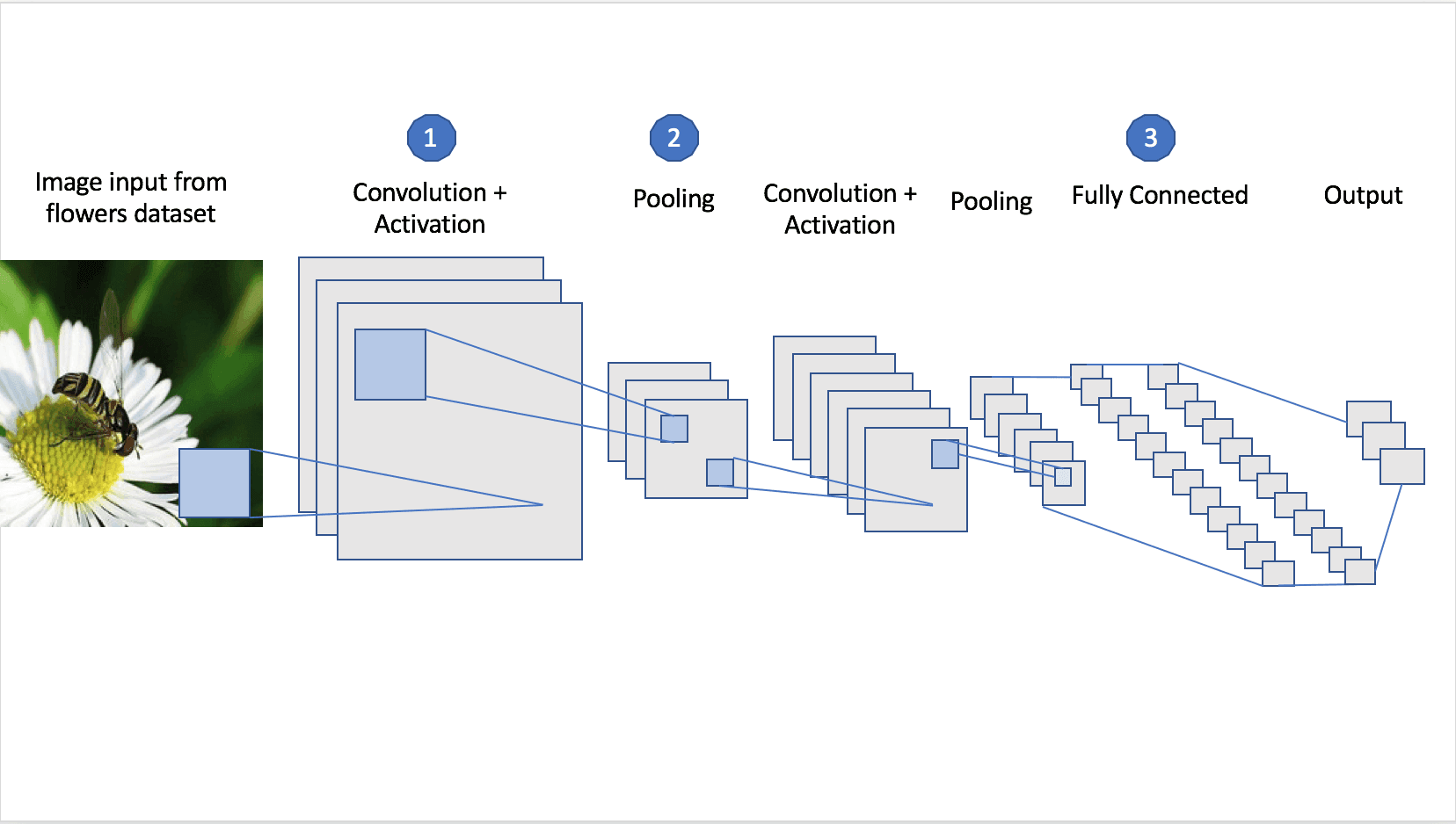
The first layer in the neural network is the convolutional (1). This is our main layer. In this step, certain effects are applied to the images, effects such as blurring or sharpening. This is achieved with filters. The filters are matrices of digits, performing matrix multiplication with the input image, resulting in a feature vector.

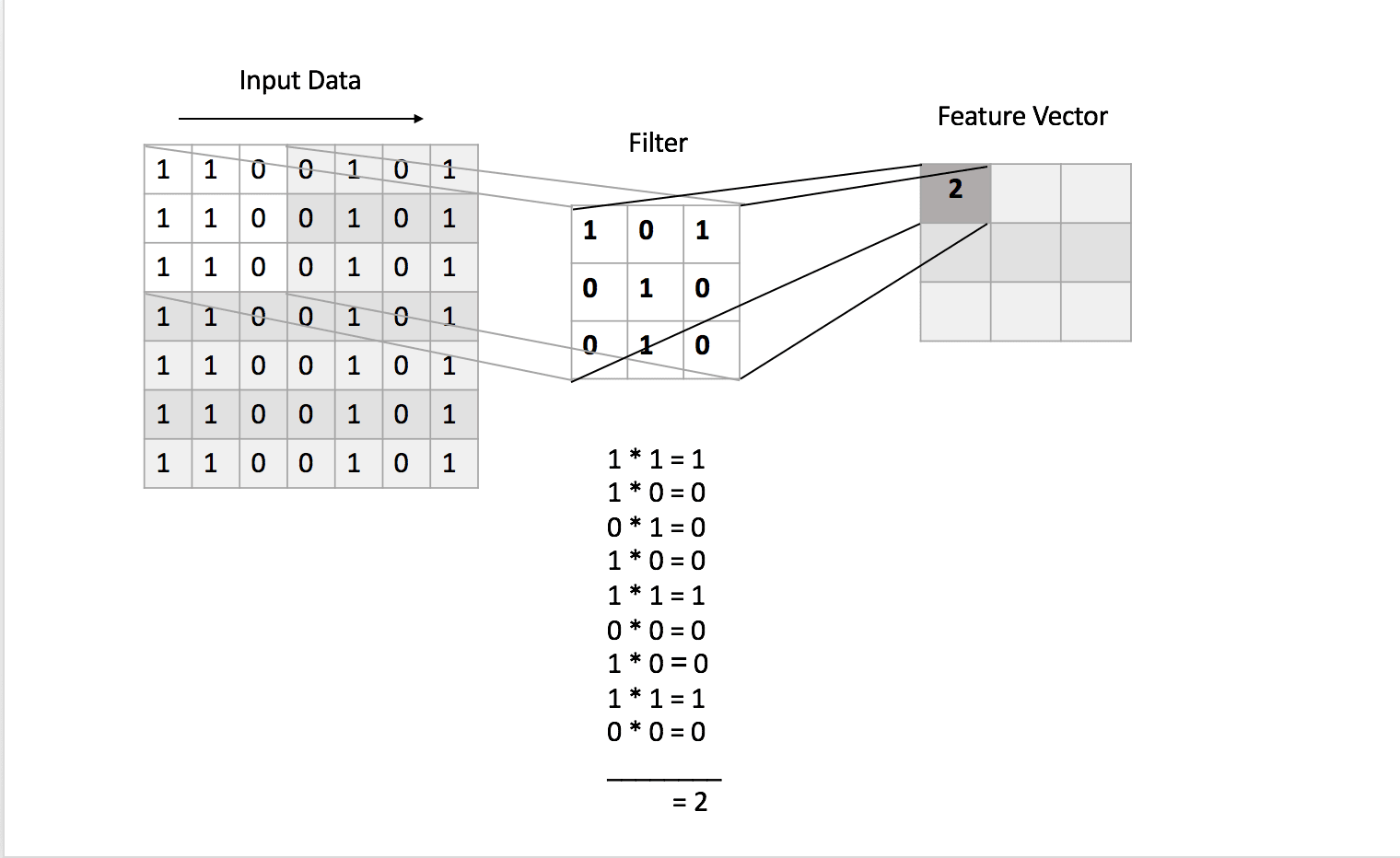
The number and size of the filters are defined by us.

The next step is dealing with the fact that the real world data is a nonlinear one. If you are not familiar with non-linearity, it is a concept where the output does not rely on the input changes. So to achieve the nonlinearity, we apply one of the activation functions available such as ReLU, sigmoid or tanh.

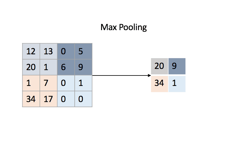
The next layer in the neural network is recommended to be the pooling layer (2). The pooling layer performs downsampling of the image input dimensions, keeping the most important features. Usually, the pooling operation can either be selecting the largest digits of the image matrix, performing a sum of the matrices numbers, or calculating the matrices average. It all depends on the type of the pooling layer.

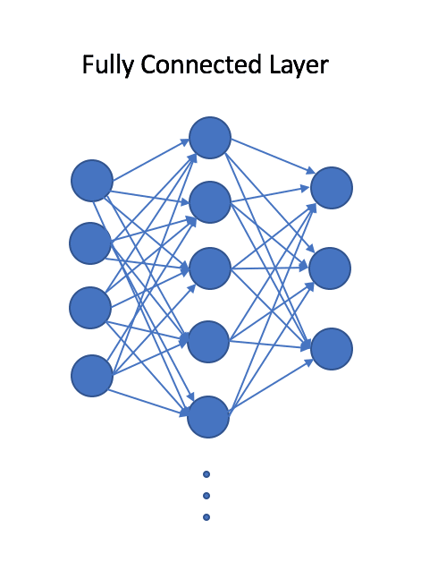
Finally, the last step of the neural network is flattening the output high dimensional matrix to a two dimensional array. Then adding the last fully connected layer in the CNN (3). This layer has connections between all the neurons and is the one responsible for performing the classification.

The dataset we will use for the training is a dataset of flowers, separated into five categories, which you can download here. One of the first problems, that was encountered with this dataset is the different dimensions of each of the images. The prerequisites for building a convolutional neural network is defining an input shape. So the first step towards processing the dataset is resizing the images. The final shape of the input is 200x200 (width x height). The following step is separating the dataset to train and test data. The threshold for test data is 20 percent. The process for resizing the images and separation can be observed below.

Project setup

First, checkout the whole code from GitHub.

Open your terminal and navigate to the folder structure where you will set the project and clone the repository. Download the folder models from this Dropbox link and place in the folder structure next to Datasets and MachineLearningTutorial folders.

In the project you can find the Python scripts for creating the neural networks for the initial training and the transfer learning.

The scripts are the following: ⋅⋅/project/algorithmFlowManager.py - Defines the flow of the scripts. ⋅⋅/project/cnn.py - Convolutional Neural Network for Initial Training ⋅⋅/project/readDataset.py - Reads the datasets ⋅⋅/project/seperateDataset.py - Separate the datasets to train and test folders. ⋅⋅/project/resizeDataset.py - Resizes the images to 200x200 dimensions. ⋅⋅/project/transferLearning.py - Convolutional Neural Network for Transfer Learning ⋅⋅/project/convertToMLModel.py - Conversion of trained model with Transfer Learning to MLModel

There are also three additional subfolders: one being datasets for the images used for training and transfer learning respectively, the other one being MachineLearningTutorial folder, where you can find the iOS Application and the last one are the trained models (downloaded from Dropbox).

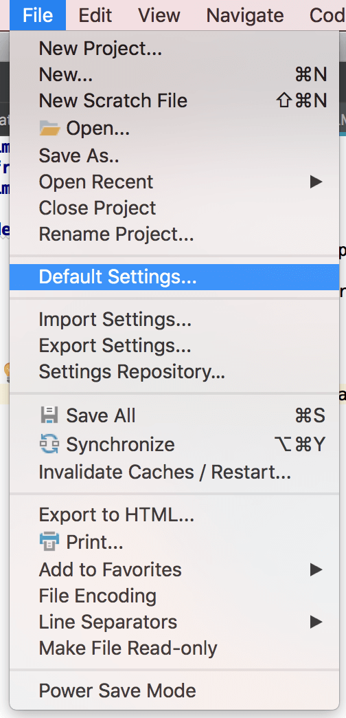
First we need to open the project, by selecting Choose File → Open . . . from the menu. The second thing during the project setup is choosing the project interpreter. To set up the interpreter open the settings options by selecting Choose File → Default Settings . . .:

You will be prompted with the window shown in the picture below. Since this will be the first time setting up the interpreter, select Project Interpreter → Add Local.

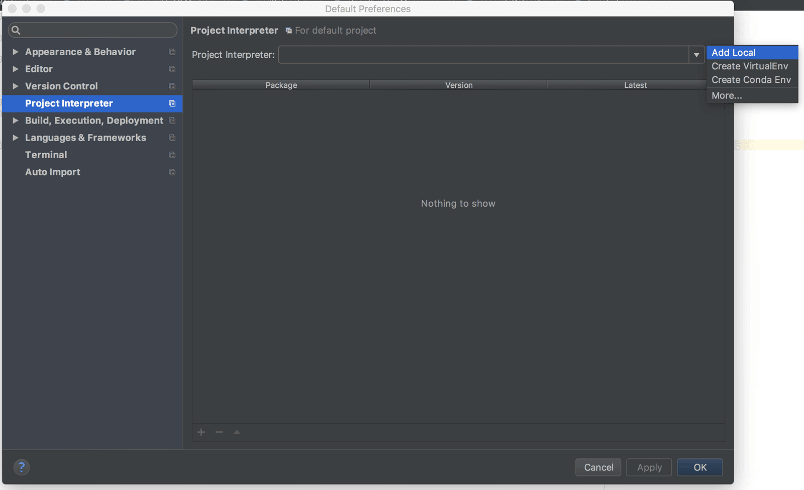
The interpreter can be found in the Miniconda or Anaconda installation folders on your computer. Usually it is located under the bin subfolder of the installation folder.

So when you set the interpreter, to check that everything works as expected, select Edit Configurations . . . . option, located next to the run button.

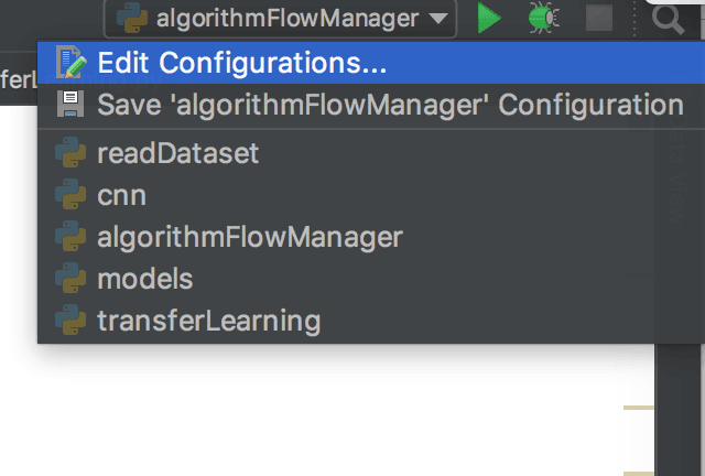
And you will get an overview for the project interpreter. Now that we are all set up, we can start working on our project.

Building the CNN

First open the script algorithmFlowManager.py.

1# ../ios-ml-app-master/algorithmFlowManager.py
2
3    import readDataset
4    import cnn
5    import transferLearning
6    import convertToMLModel
7    import seperateDataset
8    import sys
9    import os
10
11    # Returns the absolute path of the current project folder
12    def getFolderPath():
13        pathname = os.path.dirname(sys.argv[0])
14        return os.path.abspath(pathname)
15
16    trainingDir = os.path.join(getFolderPath(), "datasets","trainDataset/")
17    transferLearningDir = os.path.join(getFolderPath(), "datasets","transferLearningDataset/")
18
19    # Performs the initial training
20    def performTrainingCNN():
21        seperateDataset.createDatasetFolders(trainingDir)
22        xtrain, xtest, ytrain, ytest = readDataset.loadData(trainingDir, True)
23        modelPath = os.path.join(getFolderPath(), "models")
24        cnn.trainCNN(xtrain, xtest, ytrain, ytest, modelPath)
25
26    # Performs the transfer Learning
27    def performTransferLearning():
28        seperateDataset.createDatasetFolders(transferLearningDir)
29        xtrain, xtest, ytrain, ytest = readDataset.loadData(transferLearningDir, False)
30        modelPath = os.path.join(getFolderPath(), "models")
31        transferLearning.performTransferLearning(xtrain, xtest, ytrain, ytest, modelPath)
32
33    # Saves the trained model to .mlmodel format
34    def saveCoreMLModel():
35        convertToMLModel.convert(os.path.join(getFolderPath(), "models"))
36
37    # To start the whole process, call this function
38    def start():
39        performTrainingCNN()
40        performTransferLearning()
41        saveCoreMLModel()
42
43    start()

When calling the method:

1# ../ios-ml-app-master/algorithmFlowManager.py
2
3    def start():
4        performTrainingCNN()
5        performTransferLearning()
6        saveCoreMLModel()

We will initiate the initial training, the transfer learning and the conversion to MLModel.

If you are using macOS, you might get an error while running algorithmFlowManager.py, for unrecognized .DS_Store file in the datasets folders. To handle this run the following command:

1cd /folder
2    rm -rf .DS_Store

This will delete this file which is autogenerated Desktop Service Store, created by the Finder application on Mac.

Now we will look in the following method for the initial training:

1# ../ios-ml-app-master/algorithmFlowManager.py
2
3    def performTrainingCNN():
4        seperateDataset.createDatasetFolders(trainingDir)
5        xtrain, xtest, ytrain, ytest = readDataset.loadData(trainingDir, True)
6        modelPath = os.path.join(getFolderPath(), "models")
7        cnn.trainCNN(xtrain, xtest, ytrain, ytest, modelPath)

Looking at this method, we will notice that before training the model, the first step is to separate the dataset images to train and test subfolders.

1# ../ios-ml-app-master/algorithmFlowManager.py
2
3    seperateDataset.createDatasetFolders(trainingDir)

This method is located in seperateDataset.py script.

The next line is reading the dataset images for the corresponding folders and allocates them in arrays, such as xtrain, ytrain, xtest and ytest.

1# ../ios-ml-app-master/algorithmFlowManager.py
2
3    xtrain, xtest, ytrain, ytest = readDataset.loadData(trainingDir, True)

This method is located in readDataset.py script.

The scripts for separating the datasets and reading the data for train and test are automatically called before training of the neural network, from algorithmFlowManager.py.

Next open the script named cnn.py. Navigate to the method called from algorithmFlowManager.py:

1# ../ios-ml-app-master/cnn.py
2
3    from keras.models import Sequential
4    from keras.layers import Dense, Dropout, Flatten, Activation
5    from keras.layers import Conv2D, MaxPooling2D
6    from sklearn.model_selection import train_test_split
7    import os
8
9    def trainCNN(xtrain, xtest, ytrain, ytest, path):
10        x_train, x_validation, y_train, y_validation = train_test_split(xtrain, ytrain, 
11                                                    test_size = 0.2, random_state = 0)
12        model = Sequential()
13        model.add(Conv2D(32,(3,3), input_shape=(200,200,3)))
14        model.add(Conv2D(32,(3,3)))
15        model.add(Activation('relu'))
16        model.add(MaxPooling2D(pool_size=(2,2)))
17        model.add(Dropout(0.25))
18        model.add(Conv2D(64,(3,3)))
19        model.add(Conv2D(64, (3, 3)))
20        model.add(Activation('relu'))
21        model.add(MaxPooling2D(pool_size=(2, 2)))
22        model.add(Dropout(0.25))
23
24        model.add(Flatten())
25        model.add(Dense(128))
26        model.add(Activation('relu'))
27        model.add(Dropout(0.5))
28        model.add(Dense(5))
29        model.add(Activation('softmax'))
30
31        model.compile(loss='categorical_crossentropy',
32                  optimizer='rmsprop',
33                  metrics=['accuracy'])
34        model.fit(x_train, y_train,
35               batch_size=32, nb_epoch=10, verbose=1, validation_data=(x_validation, 
36               y_validation))
37        model.evaluate(xtest, ytest)
38        saveModel(model, path)

This method is building and training of the convolutional neural network. We will go step by step through the code.

Initially before creating the neural network, the training data is separated in train and validation datasets. The main difference between the validation and test datasets is that we use the validation dataset for fine tuning of the hyperparameters of the neural network during training, while we use the test data for evaluating the overall accuracy. The main similarity is that both of the datasets are "unknown" to the neural network.

1# ../ios-ml-app-master/cnn.py
2
3    x_train, x_validation, y_train, y_validation = train_test_split(xtrain, ytrain, 
4                                                    test_size = 0.2, random_state = 0)

When the data is separated, we will start with the creation of the model. With Keras there are two models available, Sequential and Functional. In this tutorial we will use the Sequential model.

1# ../ios-ml-app-master/cnn.py
2
3    model = Sequential()

The next step will be adding the convolutional layers. I have decided to use 32 filters in our first layer of the CNN, since it a more common practice to do so. The size of the filters will be (3,3), which is a common small size for filters, when we know that small and local features are the one that are distinctive.

Next, we will add two convolutional layers, the more convolutional layers, the better results. After the second layer, we will add activation Rectified Linear Unit (ReLU) function. The ReLU function is a nonlinear function f(x) = max(0,x), which replaces the negative values in the input with zeroes. So adding this nonlinearity is really important for the accuracy of our network. There are also other functions such as sigmoid and tanh, but this one has proved to give the best results.

1# ../ios-ml-app-master/cnn.py
2
3    model.add(Conv2D(32,(3,3), input_shape=(200,200,3)))
4    model.add(Conv2D(32,(3,3)))
5    model.add(Activation('relu'))

Next, we add the pooling layer. It is common to follow this step after convolutional layers since it reduces the number of parameters in the network and it removes the unnecessary features during the training, therefore preventing overfitting. Here we perform max pooling, which in this case is selection of the largest number in the matrix of (2,2). The pooling operation is performed on the output from the previous layer, sliding through the output matrix.

1# ../ios-ml-app-master/cnn.py
2
3    model.add(MaxPooling2D(pool_size=(2,2)))

It is recommended after the pooling layer to apply dropout, which is a regularisation technique. This technique improves the accuracy of the network by preventing inter-dependencies between the nodes. It works by randomly dropping nodes and creating new connections at each iteration of the backpropagation algorithm. This algorithm is the base of the neural network.

1# ../ios-ml-app-master/cnn.py
2
3    model.add(Dropout(0.25))

Next, we add the following convolutional layers, but with a higher number of filters, doubled because of the pooling layer.

1# ../ios-ml-app-master/cnn.py
2
3    model.add(Conv2D(64,(3,3)))
4    model.add(Conv2D(64,(3,3)))
5    model.add(Activation('relu'))
6    model.add(MaxPooling2D(pool_size=(2, 2)))
7    model.add(Dropout(0.25))

At the last stages of building our neural network, we will perform a so-called "flattening". What this does is it takes the output of the convolutional layers and flattens the higher dimension of the array to a two dimensional array. The last layer is not focused only on a limited part of the image, it needs a set of features summed from the convolution to perform the classification.

1# ../ios-ml-app-master/cnn.py
2
3    model.add(Flatten())

The dense layer is actually the fully connected layer, this means each input node is connected with each output node. The 128 is the number of neurons in this layer. It is recommended to use two dense layers since it increases the accuracy. Keep in mind that there is no perfect network topology, but with testing you can finalize your neural network structure. Here we also apply activation function.

1# ../ios-ml-app-master/cnn.py
2
3    model.add(Dense(128))
4    model.add(Activation('relu'))
5    model.add(Dropout(0.5))

The final layer is the softmax activation function which will do the classification for the images fed in the neural network.

1# ../ios-ml-app-master/cnn.py
2
3    model.add(Dense(5))
4    model.add(Activation('softmax'))

Now when we have defined our topology, we would need to compile the model. To do so, we need to define loss function. Loss function calculates the difference between the predictions of the neural network and correct answers for the dataset. The smaller the loss function, the better. There are few loss functions available, such as binary_crossentropy, Poisson, cosine_proximity, categorical_crossentropy, and sparse_categorical_crossentropy. Next, we will define the optimizer for the network, here I have chosen rmsprop, but there are also others such as adam, adagrad, adadelta, adamax and many more.

1# ../ios-ml-app-master/cnn.py
2
3    model.compile(loss='categorical_crossentropy',
4                  optimizer='rmsprop',
5                  metrics=['accuracy'])

Finally, the model is fitted with the training data for the batch size of 32 and 10 epochs. This means that the data will be iterated 10 times, and during the epoch, the images will be separated in batches of 32 until all of them are processed through the network.

1# ../ios-ml-app-master/cnn.py
2
3    model.fit(x_train, y_train,
4               batch_size=32, nb_epoch=10, verbose=1, 
5               validation_data=(x_validation, y_validation))
6    model.evaluate(xtest, ytest)

After the training of the model is finished, we need to save it. We will save the model to .h5 file format using the following method

1# ../ios-ml-app-master/cnn.py
2
3    model.save(path)

But before saving it we want to remove the last dense layers, and then set the trainable flag to the layers of the CNN to false. In the next section on transfer learning I will explain why this is done.

1# ../ios-ml-app-master/cnn.py
2
3    def saveModel(model, path):
4        layers = model.layers
5        first_dense_idx = [index for index, layer in enumerate(layers) if type(layer) is 
6        Dense][0]
7
8        num_del = len(layers) - first_dense_idx
9        for i in range(0, num_del):
10            model.pop()
11        for layer in model.layers:
12            layer.trainable = False
13
14        model.save(os.path.join(path,"model.h5"))
15        model.summary()

The following snippet is the summary of the trained model.

1# ../ios-ml-app-master/cnn.py
2
3    Layer (type)                 Output Shape              Param #   
4    =================================================================
5    conv2d_1 (Conv2D)            (None, 198, 198, 32)      896       
6    _________________________________________________________________
7    conv2d_2 (Conv2D)            (None, 196, 196, 32)      9248      
8    _________________________________________________________________
9    max_pooling2d_1 (MaxPooling2 (None, 98, 98, 32)        0         
10    _________________________________________________________________
11    dropout_1 (Dropout)          (None, 98, 98, 32)        0         
12    _________________________________________________________________
13    conv2d_3 (Conv2D)            (None, 96, 96, 64)        18496     
14    _________________________________________________________________
15    conv2d_4 (Conv2D)            (None, 94, 94, 64)        36928     
16    _________________________________________________________________
17    max_pooling2d_2 (MaxPooling2 (None, 47, 47, 64)        0         
18    _________________________________________________________________
19    dropout_2 (Dropout)          (None, 47, 47, 64)        0         
20    _________________________________________________________________
21    flatten_1 (Flatten)          (None, 141376)            0         
22    _________________________________________________________________
23    dense_1 (Dense)              (None, 128)               18096256  
24    _________________________________________________________________
25    dropout_3 (Dropout)          (None, 128)               0         
26    _________________________________________________________________
27    dense_2 (Dense)              (None, 5)                 645       
28    =================================================================
29    Total params: 18,162,469
30    Trainable params: 18,162,469
31    Non-trainable params: 0
32    _________________________________________________________________

The results of the training of the model are in the span of 95 - 99 % accuracy.

Transfer learning

Andrew Ng said "Transfer Learning will be the next driver of ML Success", and we do follow. The idea behind transfer learning is a fairly basic one. Imagine the processing power and data needed for training a powerful machine learning algorithm. Now imagine doing that for every new data, retraining the algorithm, again and again, it is nor efficient, nor fast, also we would need a lot of data. But instead of that approach, why don't we train one good neural network, save its topology and weights, load that model and remove the last layers, the one responsible for the classification of the data. Then load the saved model, add in new fully connected layers, and train this network with new data. This main difference is this data is way smaller and also we would need to train only the new layers, we will have faster and more efficient training. We have transferred the learning.

The training for the transfer learning is also intiated from algorithmFlowManger.py script.

1# ../ios-ml-app-master/algorithmFlowManager.py
2
3    def performTransferLearning():
4        seperateDataset.createDatasetFolders(transferLearningDir)
5        xtrain, xtest, ytrain, ytest = readDataset.loadData(transferLearningDir, False)
6        modelPath = os.path.join(getFolderPath(), "models")
7        transferLearning.performTransferLearning(xtrain, xtest, ytrain, ytest, modelPath)

Now to understand the algorithm for transfer learning, we will open the script transferLearning.py.

1# ../ios-ml-app-master/transferLearning.py
2
3    from keras.layers import Dense, Dropout, Activation
4    from keras.models import load_model
5    from sklearn.model_selection import train_test_split
6    import os
7
8    def performTransferLearning(xtrain, xtest, ytrain, ytest, modelPath):
9        x_train, x_validation, y_train, y_validation = train_test_split(xtrain, ytrain,
10                                                       test_size=0.2, random_state=0)
11        model = load_model(os.path.join(modelPath, "model.h5"))
12        model.add(Dense(128))
13        model.add(Activation('relu', name='activation6'))
14        model.add(Dropout(0.5, name= 'dropout4'))
15        model.add(Dense(3))
16        model.add(Activation('softmax', name='activation7'))
17
18        model.compile(loss='categorical_crossentropy',
19                      optimizer='adam', metrics=['accuracy'])
20        model.fit(x_train, y_train, validation_data=(x_validation, y_validation), epochs=30, batch_size=5)
21
22        model.evaluate(xtest, ytest)
23        # Save the model
24        model.save(os.path.join(modelPath, "transferLearning.h5"))

As you can notice, the above code is pretty familiar. We read the saved model of the trained CNN and then we add the new fully connected layers with the new number of classes.

You can notice that there is a specified name for some of the new layers, such as ‘activation6’ and ‘dropout4’, this is since the topology of the neural network can't have duplicate names. Since the loaded model already contains ‘activation1’ and ‘dropout1’. So be sure to specify these names.

The dataset I will be using for transfer learning can be downloaded from here, it is a dataset of objects, but instead of using the whole list of categories, I only used three of them for the training. The categories are a butterfly, chandelier, and hawksbill. You can also find the images attached in the datasets folder of the structure of the project. The grayscale images were also removed from the original folders since the input shape of the CNN is with three channels (RGB).

1# ../ios-ml-app-master/transferLearning.py
2
3    Layer (type)                 Output Shape              Param #   
4    =================================================================
5    conv2d_1 (Conv2D)            (None, 198, 198, 32)      896       
6    _________________________________________________________________
7    conv2d_2 (Conv2D)            (None, 196, 196, 32)      9248      
8    _________________________________________________________________
9    activation_1 (Activation)    (None, 196, 196, 32)      0         
10    _________________________________________________________________
11    max_pooling2d_1 (MaxPooling2 (None, 98, 98, 32)        0         
12    _________________________________________________________________
13    dropout_1 (Dropout)          (None, 98, 98, 32)        0         
14    _________________________________________________________________
15    conv2d_3 (Conv2D)            (None, 96, 96, 64)        18496     
16    _________________________________________________________________
17    conv2d_4 (Conv2D)            (None, 94, 94, 64)        36928     
18    _________________________________________________________________
19    activation_2 (Activation)    (None, 94, 94, 64)        0         
20    _________________________________________________________________
21    max_pooling2d_2 (MaxPooling2 (None, 47, 47, 64)        0         
22    _________________________________________________________________
23    dropout_2 (Dropout)          (None, 47, 47, 64)        0         
24    _________________________________________________________________
25    flatten_1 (Flatten)          (None, 141376)            0         
26    _________________________________________________________________
27    dense_1 (Dense)              (None, 128)               18096256  
28    _________________________________________________________________
29    activation6 (Activation)     (None, 128)               0         
30    _________________________________________________________________
31    dropout4 (Dropout)           (None, 128)               0         
32    _________________________________________________________________
33    dense_2 (Dense)              (None, 4)                 516       
34    _________________________________________________________________
35    activation7 (Activation)     (None, 4)                 0         
36    =================================================================
37    Total params: 18,162,340
38    Trainable params: 18,096,772
39    Non-trainable params: 65,568
40    _________________________________________________________________

The results of the training of the model are :

1# ../ios-ml-app-master/transferLearning.py
2
3    loss: 0.0018 - acc: 1.0000 - val_loss: 1.1946 - val_acc: 0.7692

Convert to MLModel

After we perform transfer learning we save the model and convert it into MLModel format. The conversion is called from algorithmFlowManager.py with method:

1# ../ios-ml-app-master/algorithmFlowManager.py
2
3    def saveCoreMLModel():
4        convertToMLModel.convert(os.path.join(getFolderPath(), "models"))

Open the script convertToMLModel.py. You can notice implementation of the method called from algorithmFlowManager.py.

1# ../ios-ml-app-master/convertToMLModel.py
2
3    def convert(path):
4        model = load_model(os.path.join(path, "transferLearning.h5"))
5        coreml_model = coremltools.converters.keras.convert(model,
6                                                            class_labels=['butterfly',
7                                                            'chandelier',
8                                                            'hawksbill'], 
9                                                            input_names='input_1',
10                                                            image_input_names = 'input_1')
11        coreml_model.short_description = 'Model to classify category of images'
12        coreml_model.save(os.path.join(path, "ObjectPredict.mlmodel"))

First we read the saved transfer learning model

1# ../ios-ml-app-master/convertToMLModel.py
2
3    model = load_model(os.path.join(path, "transferLearning.h5"))

Then perform the conversion by using the Python library coremltools. It supports conversion from the saved HDF5 file type to .mlmodel type, supported by Apple. Adding description to model come in handy when the MLModel is seen from the iOS Application.

1# ../ios-ml-app-master/convertToMLModel.py
2
3    coreml_model = coremltools.converters.keras.convert(model,
4                                                            class_labels=['butterfly',
5                                                            'chandelier',
6                                                            'hawksbill'], 
7                                                            input_names='input_1',
8                                                            image_input_names = 'input_1')
9    coreml_model.short_description = 'Model to classify category of images'
10    coreml_model.save(os.path.join(path, "ObjectPredict.mlmodel"))

Also before the conversion is important to add the following parameters

1# ../ios-ml-app-master/convertToMLModel.py
2
3    input_names='input_1',
4    image_input_names = 'input_1

These will allow the input for our MLModel in our iOS Application to be CVPixelBufferRef instead of MLMultiArray.

During conversion to MLModel we will see the following output:

1# ../ios-ml-app-master/convertToMLModel.py
2
3    0 : conv2d_1_input, <keras.engine.topology.InputLayer object at 0x112d094d0>
4    1 : conv2d_1, <keras.layers.convolutional.Conv2D object at 0x112d09510>
5    2 : conv2d_2, <keras.layers.convolutional.Conv2D object at 0x112d159d0>
6    3 : activation_1, <keras.layers.core.Activation object at 0x112d52910>
7    4 : max_pooling2d_1, <keras.layers.pooling.MaxPooling2D object at 0x112d52ed0>
8    5 : conv2d_3, <keras.layers.convolutional.Conv2D object at 0x112d7a710>
9    6 : conv2d_4, <keras.layers.convolutional.Conv2D object at 0x112d7a250>
10    7 : activation_2, <keras.layers.core.Activation object at 0x112dce710>
11    8 : max_pooling2d_2, <keras.layers.pooling.MaxPooling2D object at 0x112e14cd0>
12    9 : flatten_1, <keras.layers.core.Flatten object at 0x112e65b10>
13    10 : dense_1, <keras.layers.core.Dense object at 0x112db7950>
14    11 : activation6, <keras.layers.core.Activation object at 0x112e3b7d0>
15    12 : dense_2, <keras.layers.core.Dense object at 0x112ed6c90>
16    13 : activation7, <keras.layers.core.Activation object at 0x112e9ded0>

This is our first step toward building our user interface - the iOS Application.

iOS application with MLModel

Now that we have generated the ObjectPredict.ml model we need to integrate it in our iOS application. Open the MachineLearningTutorial.xcodeproj, located in MachineLearningTutorial directory, in the project we cloned, ios-ml-app-master. This will launch the Xcode interface. Next, we will drag and drop ObjectPredict.ml file in the structure folder of our project, directly in Xcode.

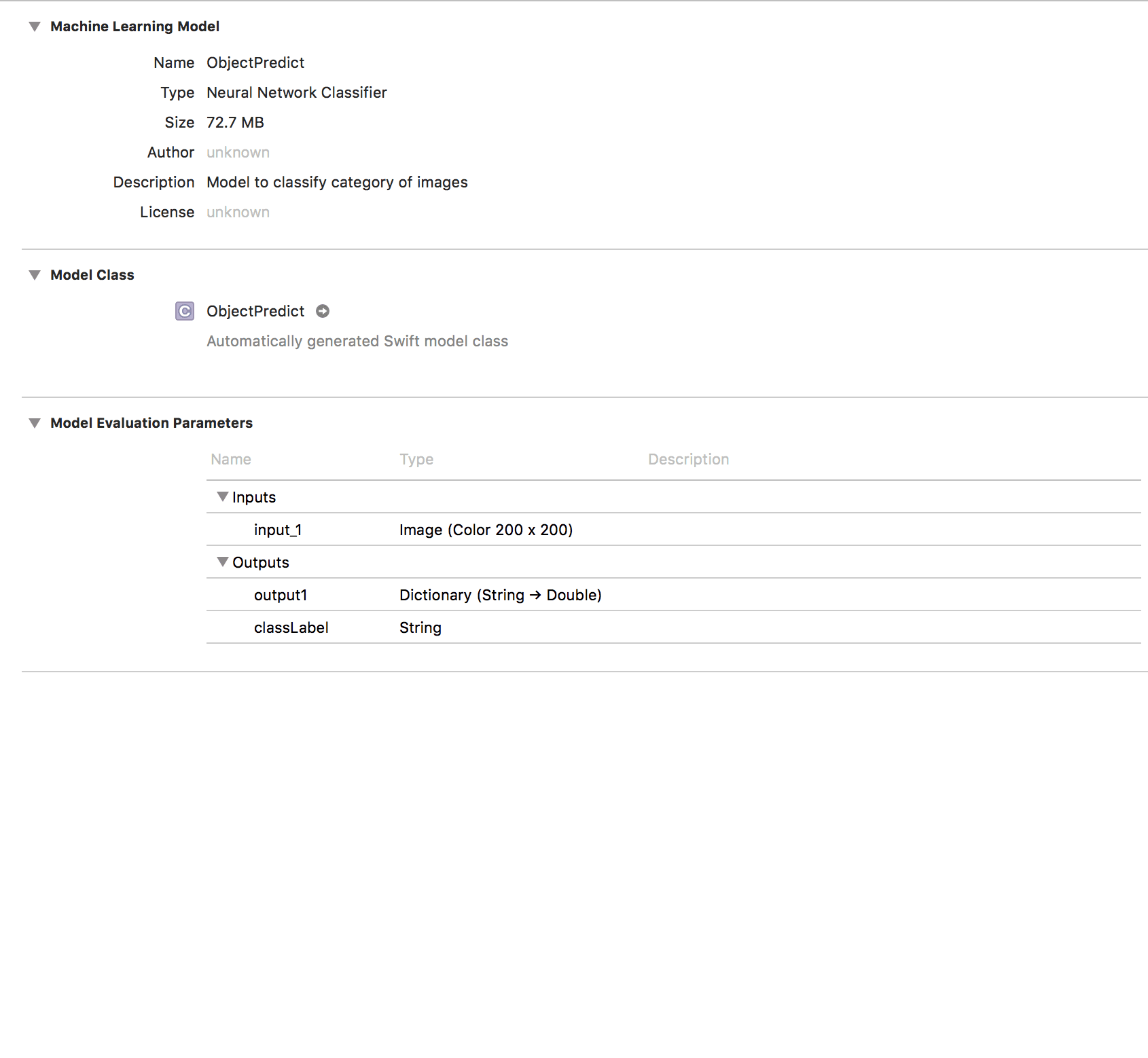
If we click on the model in XCode, it will present a generated overview of its input, output, and description.

Finally we build our application.

After a successful build, when the user selects an image, it is converted to CVPixelBuffer. This is achieved by using an open source class from GitHub which allows resizing of the image to specific dimensions and performs the conversion of the image to CVPixelBuffer. The return type of this conversion method will be the input to our MLModel Object, which will return the predicted class label.

The method responsible for the model prediction class is in the extension ViewController+Classify.swift. This method is called each time the end user choose an image.

1// ../ios-ml-app-master/MachineLearningTutorial/MachineLearningTutorial/ViewController+Classify.swift
2
3    func predictImageClass(_ image: UIImage) -> String? {
4            let model = ObjectPredict()
5            do {
6                let category = try model.prediction(input_1: image.pixelBuffer(width: 200,                                                 height: 200)!)
7                return category.classLabel
8            } catch {
9                print(error)
10                return nil
11            }
12        }

The result is being presented under the image. This can be noticed in the demo application attached above.

Tip: If you are testing on a simulator if you want to add photo in its library, just drag and drop the image and it will be automatically added.

Conclusion

So now hopefully you have a better overview of:

Collecting datasets and building a neural network
Performing transfer learning with new data (which is more than 10 times smaller in size)
And finally connecting the trained model in an iOS Application and creating a simple user interface for trying out the results.

This is the Github link from where you can access the code.

From trying out a few test images, I have noticed that for the categories that have less and more unstructured data, the results are worse. Since the accuracy of the transfer learning is not high, it can be concluded that with more and cleaner image data the neural network can learn better features from the images and show better results. Also, the initial network should have a lot more data, more epochs and bigger structure. This is why performing transfer learning on networks such as inceptionV3 created by Google Brain Team, results in high accuracy.

Hope this tutorial gave you a quick and in depth intro of what the machine learning area can do at a very small scale at least. You could also try out recurrent neural networks or their extension - LSTM, there are few examples of speech recognition that you would probably find exciting. And last but not least take up to the challenge and improve my algorithm from above, by fine tuning the parameters and improving the data, because almost always there is a more optimized version of any piece of code you will see.

References:

Transfer Learning Images - L. Fei-Fei, R. Fergus and P. Perona.
Learning generative visual models from few training examples: an incremental Bayesian approach tested on 101 object categories. IEEE. CVPR 2004, Workshop on Generative-Model Based Vision. 2004

Docs

Tutorials

Support

Glossary